![]()
![]()
Optimization of a Dissipative Quantum Gate
[1]:
# NBVAL_IGNORE_OUTPUT
%load_ext watermark
import qutip
import numpy as np
import scipy
import matplotlib
import matplotlib.pylab as plt
import krotov
import copy
from functools import partial
from itertools import product
%watermark -v --iversions
matplotlib.pylab 1.15.4
scipy            1.2.0
qutip            4.3.1
numpy            1.15.4
matplotlib       3.0.2
krotov           0.1.0.post1+dev
CPython 3.6.8
IPython 7.2.0
\(\newcommand{tr}[0]{\operatorname{tr}} \newcommand{diag}[0]{\operatorname{diag}} \newcommand{abs}[0]{\operatorname{abs}} \newcommand{pop}[0]{\operatorname{pop}} \newcommand{aux}[0]{\text{aux}} \newcommand{int}[0]{\text{int}} \newcommand{opt}[0]{\text{opt}} \newcommand{tgt}[0]{\text{tgt}} \newcommand{init}[0]{\text{init}} \newcommand{lab}[0]{\text{lab}} \newcommand{rwa}[0]{\text{rwa}} \newcommand{bra}[1]{\langle#1\vert} \newcommand{ket}[1]{\vert#1\rangle} \newcommand{Bra}[1]{\left\langle#1\right\vert} \newcommand{Ket}[1]{\left\vert#1\right\rangle} \newcommand{Braket}[2]{\left\langle #1\vphantom{#2} \mid #2\vphantom{#1}\right\rangle} \newcommand{ketbra}[2]{\vert#1\rangle\!\langle#2\vert} \newcommand{op}[1]{\hat{#1}} \newcommand{Op}[1]{\hat{#1}} \newcommand{dd}[0]{\,\text{d}} \newcommand{Liouville}[0]{\mathcal{L}} \newcommand{DynMap}[0]{\mathcal{E}} \newcommand{identity}[0]{\mathbf{1}} \newcommand{Norm}[1]{\lVert#1\rVert} \newcommand{Abs}[1]{\left\vert#1\right\vert} \newcommand{avg}[1]{\langle#1\rangle} \newcommand{Avg}[1]{\left\langle#1\right\rangle} \newcommand{AbsSq}[1]{\left\vert#1\right\vert^2} \newcommand{Re}[0]{\operatorname{Re}} \newcommand{Im}[0]{\operatorname{Im}}\)
This example illustrates the optimization for a quantum gate in an open quantum system, where the dynamics is governed by the Liouville-von Neumann equation. A naive extension of a gate optimization to Liouville space would seem to imply that it is necessary to optimize over the full basis of Liouville space (16 matrices, for a two-qubit gate). However, Goerz et al., New J. Phys. 16, 055012 (2014) [GoerzNJP2014] showed that is not necessary, but that a set of 3 density matrices is sufficient to track the optimization.
This example reproduces the “Example II” from that paper, considering the optimization towards a \(\sqrt{\text{iSWAP}}\) two-qubit gate on a system of two transmons with a shared transmission line resonator.
The two-transmon system
We consider the Hamiltonian from Eq (17) in [GoerzNJP2014], in the rotating wave approximation, together with spontaneous decay and dephasing of each qubit. Alltogether, we define the Liouvillian as follows:
[2]:
def two_qubit_transmon_liouvillian(
    ω1, ω2, ωd, δ1, δ2, J, q1T1, q2T1, q1T2, q2T2, T, Omega, n_qubit
):
    from qutip import tensor, identity, destroy

    b1 = tensor(identity(n_qubit), destroy(n_qubit))
    b2 = tensor(destroy(n_qubit), identity(n_qubit))

    H0 = (
        (ω1 - ωd - δ1 / 2) * b1.dag() * b1
        + (δ1 / 2) * b1.dag() * b1 * b1.dag() * b1
        + (ω2 - ωd - δ2 / 2) * b2.dag() * b2
        + (δ2 / 2) * b2.dag() * b2 * b2.dag() * b2
        + J * (b1.dag() * b2 + b1 * b2.dag())
    )

    H1_re = 0.5 * (b1 + b1.dag() + b2 + b2.dag())
    H1_im = 0.5j * (b1 - b1.dag() + b2 - b2.dag())

    H = [H0, [H1_re, Omega], [H1_im, ZeroPulse]]

    A1 = np.sqrt(1 / q1T1) * b1  # decay of qubit 1
    A2 = np.sqrt(1 / q2T1) * b2  # decay of qubit 2
    A3 = np.sqrt(1 / q1T2) * b1.dag() * b1  # dephasing of qubit 1
    A4 = np.sqrt(1 / q2T2) * b2.dag() * b2  # dephasing of qubit 2

    L = krotov.objectives.liouvillian(H, c_ops=[A1, A2, A3, A4])
    return L
We will use internal units GHz and ns. Values in GHz contain an implicit factor 2π, and MHz and μs are converted to GHz and ns, respectively:
[3]:
GHz = 2 * np.pi
MHz = 1e-3 * GHz
ns = 1
μs = 1000 * ns
We will use the same parameters as those given in Table 2 of [GoerzNJP2014]:
[4]:
ω1 = 4.3796 * GHz  # qubit frequency 1
ω2 = 4.6137 * GHz  # qubit frequency 2
ωd = 4.4985 * GHz  # drive frequency
δ1 = -239.3 * MHz  # anharmonicity 1
δ2 = -242.8 * MHz  # anharmonicity 2
J = -2.3 * MHz     # effective qubit-qubit coupling
q1T1 = 38.0 * μs   # decay time for qubit 1
q2T1 = 32.0 * μs   # decay time for qubit 2
q1T2 = 29.5 * μs   # dephasing time for qubit 1
q2T2 = 16.0 * μs   # dephasing time for qubit 2
T = 400 * ns       # gate duration
n_qubit = 6        # number of transmon levels to consider
[5]:
tlist = np.linspace(0, T, 2000)
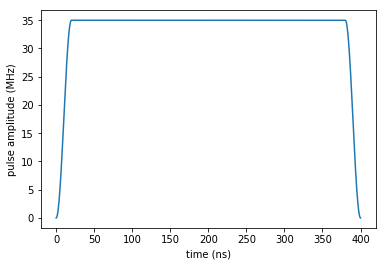
In the Liouvillian, note the control being split up into a separate real and imaginary part. As a guess control we use a real-valued constant pulse with and amplitude of 35 MHz, acting over 400 ns, with a switch-on and switch-off in the first 20 ns (see plot below)
[6]:
def Omega(t, args):
    E0 = 35.0 * MHz
    return E0 * krotov.shapes.flattop(t, 0, T, t_rise=(20 * ns), func='sinsq')
The imaginary part start out as zero:
[7]:
def ZeroPulse(t, args):
    return 0.0
We can now instantiate the Liouvillian:
[8]:
L = two_qubit_transmon_liouvillian(
    ω1, ω2, ωd, δ1, δ2, J, q1T1, q2T1, q1T2, q2T2, T, Omega, n_qubit
)
The guess pulse looks as follows:
[9]:
def plot_pulse(pulse, tlist, xlimit=None):
    fig, ax = plt.subplots()
    if callable(pulse):
        pulse = np.array([pulse(t, None) for t in tlist])
    ax.plot(tlist, pulse/MHz)
    ax.set_xlabel('time (ns)')
    ax.set_ylabel('pulse amplitude (MHz)')
    if xlimit is not None:
        ax.set_xlim(xlimit)
    plt.show(fig)
[10]:
plot_pulse(L[1][1], tlist)
Optimization objectives
Our target gate is \(\sqrt{\text{iSWAP}}\):
[11]:
gate = qutip.gates.sqrtiswap()
[12]:
gate
[12]:
The key idea explored in [GoerzNJP2014] is that a set of three density matrices is sufficient to track the optimization
:nbsphinx-math:`begin{align} Op{rho}_1 &= sum_{i=1}^{d}
frac{2 (d-i+1)}{d (d+1)} ketbra{i}{i} \
- Op{rho}_2 &= sum_{i,j=1}^{d}
- frac{1}{d} ketbra{i}{j} \
- Op{rho}_3 &= sum_{i=1}^{d}
- frac{1}{d} ketbra{i}{i}
end{align}`
In our case, \(d=4\) for a two qubit-gate, and the \(\ket{i}\), \(\ket{j}\) are the canonical basis states \(\ket{00}\), \(\ket{01}\), \(\ket{10}\), \(\ket{11}\)
[13]:
ket00 = qutip.ket((0, 0), dim=(n_qubit, n_qubit))
ket01 = qutip.ket((0, 1), dim=(n_qubit, n_qubit))
ket10 = qutip.ket((1, 0), dim=(n_qubit, n_qubit))
ket11 = qutip.ket((1, 1), dim=(n_qubit, n_qubit))
basis = [ket00, ket01, ket10, ket11]
The three density matrices play different roles in the optimization, and, as shown in [GoerzNJP2014], convergence may improve significantly by weighing the states relatively to each other. For this example, we place a strong emphasis on the optimization \(\Op{\rho}_1 \rightarrow \Op{O}^\dagger \Op{\rho}_1 \Op{O}\), by a factor of 20. This reflects that the hardest part of the optimization is identifying the basis in which the gate is diagonal.
[14]:
weights = [20, 1, 1]
The krotov.gate_objectives routine can initialize the density matrices \(\Op{\rho}_1\), \(\Op{\rho}_2\), \(\Op{\rho}_3\) automatically, via the parameter liouville_states_set. Alternatively, we could also use the 'full' basis of 16 matrices or the extended set of \(d+1 = 5\) pure-state density matrices.
[15]:
objectives = krotov.gate_objectives(basis, gate, L, liouville_states_set='3states', weights=weights)
The weights are automatically normalized and stored in the weight attribute of the three objectives:
[16]:
for obj in objectives:
    print("%.5f" % obj.weight)
2.72727
0.13636
0.13636
Dynamics under the Guess Pulse
For numerical efficiency, both for the analysis of the guess/optimized controls, we will use a stateful density matrix propagator:
[17]:
propagator = krotov.propagators.DensityMatrixODEPropagator()
A true physical measure for the success of the optimization is the “average gate fidelity”. Evaluating the fidelity requires to simulate the dynamics of the full basis of Liouville space:
[18]:
full_liouville_basis = [psi * phi.dag() for (psi, phi) in product(basis, basis)]
We propagate these under the guess control:
[19]:
def propagate_guess(initial_state):
    return objectives[0].propagate(
        tlist,
        propagator=propagator,
        rho0=initial_state,
    ).states[-1]
[20]:
full_states_T = qutip.parallel_map(
    propagate_guess, values=full_liouville_basis,
)
[21]:
print("F_avg = %.3f" % krotov.functionals.F_avg(full_states_T, basis, gate))
F_avg = 0.344
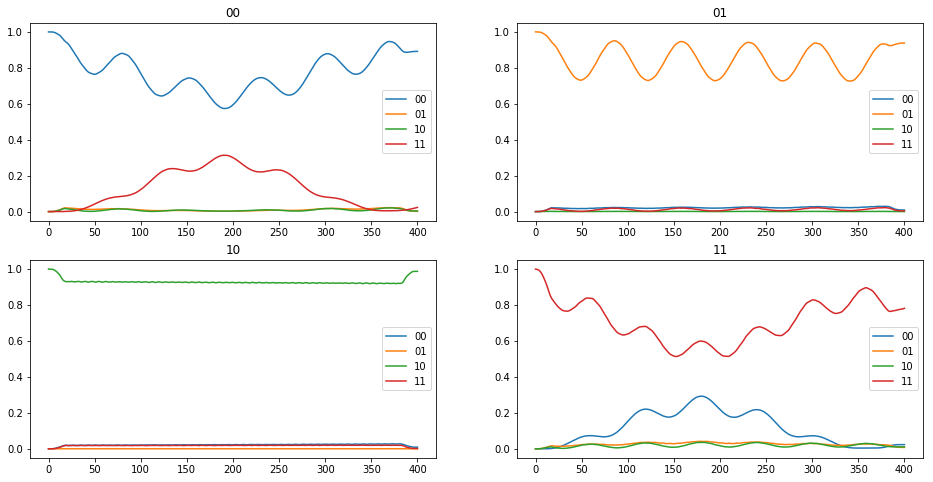
We can also consider the population dynamics, under the guess pulse. For this purpose we propagate the pure-state density matrices corresponding to the canonical logical basis in Hilbert space, and obtain the expectation values for the projection onto these same states:
[22]:
rho00, rho01, rho10, rho11 = [qutip.ket2dm(psi) for psi in basis]
[23]:
def propagate_guess_for_expvals(initial_state):
    return objectives[0].propagate(
        tlist,
        propagator=propagator,
        rho0=initial_state,
        e_ops=[rho00, rho01, rho10, rho11]
    )
[24]:
def plot_population_dynamics(dyn00, dyn01, dyn10, dyn11):
    fig, axs = plt.subplots(ncols=2, nrows=2, figsize=(16, 8))
    axs = np.ndarray.flatten(axs)
    labels = ['00', '01', '10', '11']
    dyns = [dyn00, dyn01, dyn10, dyn11]
    for (ax, dyn, title) in zip(axs, dyns, labels):
        for (i, label) in enumerate(labels):
            ax.plot(dyn.times, dyn.expect[i], label=label)
        ax.legend()
        ax.set_title(title)
    plt.show(fig)
[25]:
plot_population_dynamics(
    *qutip.parallel_map(
        propagate_guess_for_expvals,
        values=[rho00, rho01, rho10, rho11],
    )
)
Optimization
Before running the optimizaton, we have to define the optimization parameters for the controls, the Krotov step size \(\lambda_a\) and the update-shape that will ensure that the pulse switch-on and switch-off stays intact.
[26]:
pulse_options = {
    L[i][1]: dict(
        lambda_a=1.0,
        shape=partial(
            krotov.shapes.flattop, t_start=0, t_stop=T, t_rise=(20 * ns))
        )
    for i in [1, 2]
}
[27]:
import logging
logger = logging.getLogger()
logger.setLevel(logging.DEBUG)
ch = logging.StreamHandler()
ch.setLevel(logging.DEBUG)
formatter = logging.Formatter("%(asctime)s:%(message)s")
ch.setFormatter(formatter)
logger.handlers = []
logger.addHandler(ch)
[28]:
def print_error(**args):
    J_T_hs = krotov.functionals.J_T_hs(
        args['fw_states_T'], args['objectives'], args['tau_vals']
    )
    print("Iteration %d: \tJ_T_hs = %f" % (args['iteration'], J_T_hs))
    return J_T_hs
[29]:
# NBVAL_SKIP
oct_result = krotov.optimize_pulses(
    objectives,
    pulse_options,
    tlist,
    propagator=propagator,
    chi_constructor=krotov.functionals.chis_hs,
    info_hook=print_error,
    iter_stop=5,
    #parallel_map=(
    #    qutip.parallel_map,
    #    qutip.parallel_map,
    #    krotov.parallelization.parallel_map_fw_prop_step,
    #),
)
2019-02-11 02:03:26,073:Initializing optimization with Krotov's method
2019-02-11 02:03:26,112:Started initial forward propagation of objective 0
2019-02-11 02:03:40,671:Finished initial forward propagation of objective 0
2019-02-11 02:03:40,672:Started initial forward propagation of objective 1
2019-02-11 02:03:52,199:Finished initial forward propagation of objective 1
2019-02-11 02:03:52,199:Started initial forward propagation of objective 2
2019-02-11 02:04:04,405:Finished initial forward propagation of objective 2
2019-02-11 02:04:04,408:Started Krotov iteration 1
2019-02-11 02:04:04,415:Started backward propagation of state 0
Iteration 0: J_T_hs = 0.063449
2019-02-11 02:04:12,823:Finished backward propagation of state 0
2019-02-11 02:04:12,824:Started backward propagation of state 1
2019-02-11 02:04:21,094:Finished backward propagation of state 1
2019-02-11 02:04:21,095:Started backward propagation of state 2
2019-02-11 02:04:30,908:Finished backward propagation of state 2
2019-02-11 02:04:30,909:Started forward propagation/pulse update
---------------------------------------------------------------------------
IntegratorConcurrencyError                Traceback (most recent call last)
<ipython-input-29-f13f2354e6c9> in <module>
      7     chi_constructor=krotov.functionals.chis_hs,
      8     info_hook=print_error,
----> 9     iter_stop=5,
     10     #parallel_map=(
     11     #    qutip.parallel_map,

~/Documents/Programming/github/krotov/src/krotov/optimize.py in optimize_pulses(objectives, pulse_options, tlist, propagator, chi_constructor, mu, sigma, iter_start, iter_stop, check_convergence, state_dependent_constraint, info_hook, modify_params_after_iter, storage, parallel_map, store_all_pulses)
    349                     tlist,
    350                     time_index,
--> 351                     propagators,
    352                 ),
    353             )

~/Documents/Programming/github/krotov/.venv/py36/lib/python3.6/site-packages/qutip/parallel.py in serial_map(task, values, task_args, task_kwargs, **kwargs)
    181     for n, value in enumerate(values):
    182         progress_bar.update(n)
--> 183         result = task(value, *task_args, **task_kwargs)
    184         results.append(result)
    185     progress_bar.finished()

~/Documents/Programming/github/krotov/src/krotov/optimize.py in _forward_propagation_step(i_state, states, objectives, pulses, pulses_mapping, tlist, time_index, propagators)
    623     dt = tlist[time_index + 1] - tlist[time_index]
    624     return propagators[i_state](
--> 625         H, state, dt, c_ops, initialize=(time_index == 0)
    626     )

~/Documents/Programming/github/krotov/src/krotov/propagators.py in __call__(self, L, rho, dt, c_ops, backwards, initialize)
    152                 self._L_list[i][1] = L[i][1]
    153         self._t += dt
--> 154         self._r.integrate(self._t)
    155         return qutip.Qobj(
    156             dense2D_to_fastcsr_fmode(

~/Documents/Programming/github/krotov/.venv/py36/lib/python3.6/site-packages/scipy/integrate/_ode.py in integrate(self, t, step, relax)
    430             self._y, self.t = mth(self.f, self.jac or (lambda: None),
    431                                   self._y, self.t, t,
--> 432                                   self.f_params, self.jac_params)
    433         except SystemError:
    434             # f2py issue with tuple returns, see ticket 1187.

~/Documents/Programming/github/krotov/.venv/py36/lib/python3.6/site-packages/scipy/integrate/_ode.py in run(self, f, jac, y0, t0, t1, f_params, jac_params)
    989     def run(self, f, jac, y0, t0, t1, f_params, jac_params):
    990         if self.initialized:
--> 991             self.check_handle()
    992         else:
    993             self.initialized = True

~/Documents/Programming/github/krotov/.venv/py36/lib/python3.6/site-packages/scipy/integrate/_ode.py in check_handle(self)
    789     def check_handle(self):
    790         if self.handle is not self.__class__.active_global_handle:
--> 791             raise IntegratorConcurrencyError(self.__class__.__name__)
    792
    793     def reset(self, n, has_jac):

IntegratorConcurrencyError: Integrator `zvode` can be used to solve only a single problem at a time. If you want to integrate multiple problems, consider using a different integrator (see `ode.set_integrator`)