![]()
![]()
Optimization of an X-Gate for a Transmon Qubit
[1]:
# NBVAL_IGNORE_OUTPUT
%load_ext watermark
import sys
import os
import qutip
import numpy as np
import scipy
import matplotlib
import matplotlib.pylab as plt
import krotov
from scipy.fftpack import fft
from scipy.interpolate import interp1d
%watermark -v --iversions
krotov           1.2.0
matplotlib.pylab 1.17.2
matplotlib       3.3.1
scipy            1.3.1
qutip            4.5.0
numpy            1.17.2
CPython 3.7.6
IPython 7.17.0
\(\newcommand{tr}[0]{\operatorname{tr}} \newcommand{diag}[0]{\operatorname{diag}} \newcommand{abs}[0]{\operatorname{abs}} \newcommand{pop}[0]{\operatorname{pop}} \newcommand{aux}[0]{\text{aux}} \newcommand{opt}[0]{\text{opt}} \newcommand{tgt}[0]{\text{tgt}} \newcommand{init}[0]{\text{init}} \newcommand{lab}[0]{\text{lab}} \newcommand{rwa}[0]{\text{rwa}} \newcommand{bra}[1]{\langle#1\vert} \newcommand{ket}[1]{\vert#1\rangle} \newcommand{Bra}[1]{\left\langle#1\right\vert} \newcommand{Ket}[1]{\left\vert#1\right\rangle} \newcommand{Braket}[2]{\left\langle #1\vphantom{#2} \mid #2\vphantom{#1}\right\rangle} \newcommand{op}[1]{\hat{#1}} \newcommand{Op}[1]{\hat{#1}} \newcommand{dd}[0]{\,\text{d}} \newcommand{Liouville}[0]{\mathcal{L}} \newcommand{DynMap}[0]{\mathcal{E}} \newcommand{identity}[0]{\mathbf{1}} \newcommand{Norm}[1]{\lVert#1\rVert} \newcommand{Abs}[1]{\left\vert#1\right\vert} \newcommand{avg}[1]{\langle#1\rangle} \newcommand{Avg}[1]{\left\langle#1\right\rangle} \newcommand{AbsSq}[1]{\left\vert#1\right\vert^2} \newcommand{Re}[0]{\operatorname{Re}} \newcommand{Im}[0]{\operatorname{Im}}\)
In the previous examples, we have only optimized for state-to-state transitions, i.e., for a single objective. This example shows the optimization of a simple quantum gate, which requires multiple objectives to be fulfilled simultaneously (one for each state in the logical basis). We consider a superconducting “transmon” qubit and implement a single-qubit Pauli-X gate.
Note: This notebook uses some parallelization features (parallel_map/multiprocessing). Unfortunately, on Windows (and macOS with Python >= 3.8), multiprocessing does not work correctly for functions defined in a Jupyter notebook (due to the spawn method being used on Windows, instead of Unix-fork, see also https://stackoverflow.com/questions/45719956). We can use the third-party
loky library to fix this, but this significantly increases the overhead of multi-process parallelization. The use of parallelization here is for illustration only and makes no guarantee of actually improving the runtime of the optimization.
[2]:
krotov.parallelization.set_parallelization(use_loky=True)
The transmon Hamiltonian
The effective Hamiltonian of a single transmon depends on the capacitive energy \(E_C=e^2/2C\) and the Josephson energy \(E_J\), an energy due to the Josephson junction working as a nonlinear inductor periodic with the flux \(\Phi\). In the so-called transmon limit, the ratio between these two energies lies around \(E_J / E_C \approx 45\). The Hamiltonian for the transmon is
where \(\hat{n}\) is the number operator, which counts the relative number of Cooper pairs capacitively stored in the junction, and \(n_g\) is the effective offset charge measured in Cooper pair charge units. The equation can be written in a truncated charge basis defined by the number operator \(\op{n} \ket{n} = n \ket{n}\) such that
A voltage \(V(t)\) applied to the circuit couples to the charge Hamiltonian \(\op{q}\), which in the (truncated) charge basis reads
The factor 2 is due to the charge carriers in a superconductor being Cooper pairs. The total Hamiltonian is
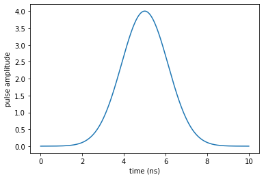
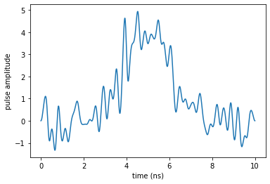
We use a Gaussian voltage profile as the guess pulse:
[3]:
tlist = np.linspace(0, 10, 1000)

def eps0(t, args):
    T = tlist[-1]
    return 4 * np.exp(-40.0 * (t / T - 0.5) ** 2)
[4]:
def plot_pulse(pulse, tlist, xlimit=None):
    fig, ax = plt.subplots()
    if callable(pulse):
        pulse = np.array([pulse(t, None) for t in tlist])
    ax.plot(tlist, pulse)
    ax.set_xlabel('time (ns)')
    ax.set_ylabel('pulse amplitude')
    if xlimit is not None:
        ax.set_xlim(xlimit)
    plt.show(fig)
[5]:
plot_pulse(eps0, tlist)
The complete Hamiltonian is instantiated as
[6]:
def transmon_hamiltonian(Ec=0.386, EjEc=45, nstates=8, ng=0.0, T=10.0):
    """Transmon Hamiltonian

    Args:
        Ec: capacitive energy
        EjEc: ratio `Ej` / `Ec`
        nstates: defines the maximum and minimum states for the basis. The
            truncated basis will have a total of ``2*nstates + 1`` states

        ng: offset charge
        T: gate duration
    """

    Ej = EjEc * Ec
    n = np.arange(-nstates, nstates + 1)
    up = np.diag(np.ones(2 * nstates), k=-1)
    do = up.T
    H0 = qutip.Qobj(np.diag(4 * Ec * (n - ng) ** 2) - Ej * (up + do) / 2.0)
    H1 = qutip.Qobj(-2 * np.diag(n))

    return [H0, [H1, eps0]]
[7]:
H = transmon_hamiltonian()
We define the logical basis \(\ket{0_l}\) and \(\ket{1_l}\) (not to be confused with the charge states \(\ket{n=0}\) and \(\ket{n=1}\)) as the eigenstates of the drift Hamiltonian \(\op{H}_0\) with the lowest energy. The optimization goal is to find a potential \(V_{opt}(t)\) such that after a given final time \(T\) implements an X-gate on this logical basis.
[8]:
def logical_basis(H):
    H0 = H[0]
    eigenvals, eigenvecs = scipy.linalg.eig(H0.full())
    ndx = np.argsort(eigenvals.real)
    E = eigenvals[ndx].real
    V = eigenvecs[:, ndx]
    psi0 = qutip.Qobj(V[:, 0])
    psi1 = qutip.Qobj(V[:, 1])
    w01 = E[1] - E[0]  # Transition energy between states
    print("Energy of qubit transition is %.3f" % w01)
    return psi0, psi1

psi0, psi1 = logical_basis(H)
Energy of qubit transition is 6.914
We also introduce the projectors \(P_i = \ket{\psi _i}\bra{\psi _i}\) for the logical states \(\ket{\psi _i} \in \{\ket{0_l}, \ket{1_l}\}\)
[9]:
proj0 = qutip.ket2dm(psi0)
proj1 = qutip.ket2dm(psi1)
Optimization target
The key insight for the realization of a quantum gate \(\Op{O}\) is that (by virtue of linearity)
is fulfilled for an arbitrary state \(\Ket{\Psi(t=0)}\) if an only if \(\Op{U}(T, \epsilon(t))\ket{k} = \Op{O} \ket{k}\) for every state \(\ket{k}\) in logical basis, for the time evolution operator \(\Op{U}(T, \epsilon(t))\) from \(t=0\) to \(t=T\) under the same control \(\epsilon(t)\).
The function krotov.gate_objectives automatically sets up the corresponding objectives \(\forall \ket{k}: \ket{k} \rightarrow \Op{O} \ket{k}\):
[10]:
objectives = krotov.gate_objectives(
    basis_states=[psi0, psi1], gate=qutip.operators.sigmax(), H=H
)

objectives
[10]:
[Objective[|Ψ₀(17)⟩ to |Ψ₁(17)⟩ via [H₀[17,17], [H₁[17,17], u₁(t)]]],
 Objective[|Ψ₁(17)⟩ to |Ψ₀(17)⟩ via [H₀[17,17], [H₁[17,17], u₁(t)]]]]
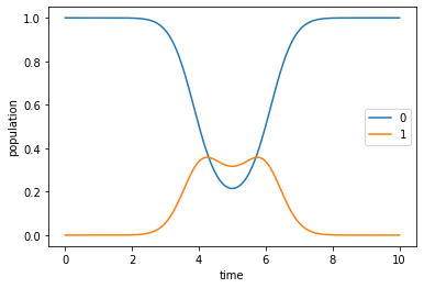
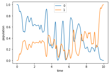
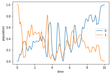
Dynamics of the guess pulse
[11]:
guess_dynamics = [
    objectives[x].mesolve(tlist, e_ops=[proj0, proj1]) for x in [0, 1]
]
[12]:
def plot_population(result):
    '''Representation of the expected values for the initial states'''
    fig, ax = plt.subplots()
    ax.plot(result.times, result.expect[0], label='0')
    ax.plot(result.times, result.expect[1], label='1')
    ax.legend()
    ax.set_xlabel('time')
    ax.set_ylabel('population')
    plt.show(fig)
[13]:
plot_population(guess_dynamics[0])
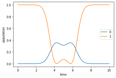
plot_population(guess_dynamics[1])
Optimization
We define the desired shape of the update and the factor \(\lambda_a\), and then start the optimization
[14]:
def S(t):
    """Scales the Krotov methods update of the pulse value at the time t"""
    return krotov.shapes.flattop(
        t, t_start=0.0, t_stop=10.0, t_rise=0.5, func='sinsq'
    )

pulse_options = {H[1][1]: dict(lambda_a=1, update_shape=S)}
[15]:
opt_result = krotov.optimize_pulses(
    objectives,
    pulse_options,
    tlist,
    propagator=krotov.propagators.expm,
    chi_constructor=krotov.functionals.chis_re,
    info_hook=krotov.info_hooks.print_table(
        J_T=krotov.functionals.J_T_re,
        show_g_a_int_per_pulse=True,
        unicode=False,
    ),
    check_convergence=krotov.convergence.Or(
        krotov.convergence.value_below(1e-3, name='J_T'),
        krotov.convergence.delta_below(1e-5),
        krotov.convergence.check_monotonic_error,
    ),
    iter_stop=5,
    parallel_map=(
        krotov.parallelization.parallel_map,
        krotov.parallelization.parallel_map,
        krotov.parallelization.parallel_map_fw_prop_step,
    ),
)
iter.      J_T    g_a_int          J  Delta J_T    Delta J  secs
0     1.00e+00   0.00e+00   1.00e+00        n/a        n/a    11
1     2.80e-01   3.41e-01   6.22e-01  -7.20e-01  -3.78e-01    23
2     2.12e-01   3.06e-02   2.43e-01  -6.81e-02  -3.75e-02    21
3     1.35e-01   3.28e-02   1.68e-01  -7.72e-02  -4.44e-02    23
4     9.79e-02   1.56e-02   1.13e-01  -3.71e-02  -2.15e-02    22
5     7.13e-02   1.11e-02   8.25e-02  -2.65e-02  -1.54e-02    21
(this takes a while …)
[16]:
dumpfile = "./transmonxgate_opt_result.dump"
if os.path.isfile(dumpfile):
    opt_result = krotov.result.Result.load(dumpfile, objectives)
else:
    opt_result = krotov.optimize_pulses(
        objectives,
        pulse_options,
        tlist,
        propagator=krotov.propagators.expm,
        chi_constructor=krotov.functionals.chis_re,
        info_hook=krotov.info_hooks.print_table(
            J_T=krotov.functionals.J_T_re,
            show_g_a_int_per_pulse=True,
            unicode=False,
        ),
        check_convergence=krotov.convergence.Or(
            krotov.convergence.value_below(1e-3, name='J_T'),
            krotov.convergence.delta_below(1e-5),
            krotov.convergence.check_monotonic_error,
        ),
        iter_stop=1000,
        parallel_map=(
            qutip.parallel_map,
            qutip.parallel_map,
            krotov.parallelization.parallel_map_fw_prop_step,
        ),
        continue_from=opt_result
    )
    opt_result.dump(dumpfile)
[17]:
opt_result
[17]:
Krotov Optimization Result
--------------------------
- Started at 2019-04-12 17:45:43
- Number of objectives: 2
- Number of iterations: 398
- Reason for termination: Reached convergence: Δ(('info_vals', T[-1]),('info_vals', T[-2])) < 1e-05
- Ended at 2019-04-12 18:20:47 (0:35:04)
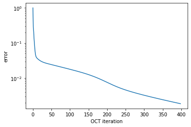
[18]:
def plot_convergence(result):
    fig, ax = plt.subplots()
    ax.semilogy(result.iters, np.array(result.info_vals))
    ax.set_xlabel('OCT iteration')
    ax.set_ylabel('error')
    plt.show(fig)
[19]:
plot_convergence(opt_result)
Optimized pulse and dynamics
We obtain the following optimized pulse:
[20]:
plot_pulse(opt_result.optimized_controls[0], tlist)
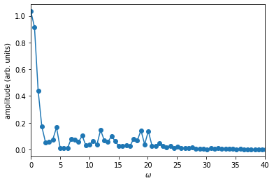
The oscillations in the control shape indicate non-negligible spectral broadening:
[21]:
def plot_spectrum(pulse, tlist, xlim=None):

    if callable(pulse):
        pulse = np.array([pulse(t, None) for t in tlist])

    dt = tlist[1] - tlist[0]
    n = len(tlist)

    w = np.fft.fftfreq(n, d=dt/(2.0*np.pi))
    # the factor 2π in the normalization means that
    # the spectrum is in units of angular frequency,
    # which is normally what we want

    spectrum = np.fft.fft(pulse) / n
    # normalizing the spectrum with n means that
    # the y-axis is independent of dt

    # we assume a real-valued pulse, so we throw away
    # the half of the spectrum with negative frequencies
    w = w[range(int(n / 2))]
    spectrum = np.abs(spectrum[range(int(n / 2))])

    fig, ax = plt.subplots()
    ax.plot(w, spectrum, '-o')
    ax.set_xlabel(r'$\omega$')
    ax.set_ylabel('amplitude (arb. units)')
    if xlim is not None:
        ax.set_xlim(*xlim)
    plt.show(fig)


plot_spectrum(opt_result.optimized_controls[0], tlist, xlim=(0, 40))
Lastly, we verify that the pulse produces the desired dynamics \(\ket{0_l} \rightarrow \ket{1_l}\) and \(\ket{1_l} \rightarrow \ket{0_l}\):
[22]:
opt_dynamics = [
    opt_result.optimized_objectives[x].mesolve(tlist, e_ops=[proj0, proj1])
    for x in [0, 1]
]
[23]:
plot_population(opt_dynamics[0])
[24]:
plot_population(opt_dynamics[1])
Since the optimized pulse shows some oscillations (cf. the spectrum above), it is a good idea to check for any discretization error. To this end, we also propagate the optimization result using the same propagator that was used in the optimization (instead of qutip.mesolve). The main difference between the two propagations is that mesolve assumes piecewise constant pulses that switch between two points in tlist, whereas propagate assumes that pulses are constant on the intervals
of tlist, and thus switches on the points in tlist.
[25]:
opt_dynamics2 = [
    opt_result.optimized_objectives[x].propagate(
        tlist, e_ops=[proj0, proj1], propagator=krotov.propagators.expm
    )
    for x in [0, 1]
]
The difference between the two propagations gives an indication of the error due to the choice of the piecewise constant time discretization. If this error were unacceptably large, we would need a smaller time step.
[26]:
# NBVAL_IGNORE_OUTPUT
# Note: the particular error value may depend on the version of QuTiP
print(
    "Time discretization error = %.1e" %
    abs(opt_dynamics2[0].expect[1][-1] - opt_dynamics[0].expect[1][-1])
)
Time discretization error = 2.9e-05