Optimization with numpy Arrays

# NBVAL_IGNORE_OUTPUT
%load_ext watermark
import numpy as np
import scipy
import matplotlib
import matplotlib.pylab as plt
import krotov
# note that qutip is NOT imported
%watermark -v --iversions

numpy            1.17.2
scipy            1.3.1
matplotlib       3.1.2
krotov           1.0.0
matplotlib.pylab 1.17.2
CPython 3.7.3
IPython 7.10.2

\(\newcommand{tr}[0]{\operatorname{tr}} \newcommand{diag}[0]{\operatorname{diag}} \newcommand{abs}[0]{\operatorname{abs}} \newcommand{pop}[0]{\operatorname{pop}} \newcommand{aux}[0]{\text{aux}} \newcommand{opt}[0]{\text{opt}} \newcommand{tgt}[0]{\text{tgt}} \newcommand{init}[0]{\text{init}} \newcommand{lab}[0]{\text{lab}} \newcommand{rwa}[0]{\text{rwa}} \newcommand{bra}[1]{\langle#1\vert} \newcommand{ket}[1]{\vert#1\rangle} \newcommand{Bra}[1]{\left\langle#1\right\vert} \newcommand{Ket}[1]{\left\vert#1\right\rangle} \newcommand{Braket}[2]{\left\langle #1\vphantom{#2} \mid #2\vphantom{#1}\right\rangle} \newcommand{op}[1]{\hat{#1}} \newcommand{Op}[1]{\hat{#1}} \newcommand{dd}[0]{\,\text{d}} \newcommand{Liouville}[0]{\mathcal{L}} \newcommand{DynMap}[0]{\mathcal{E}} \newcommand{identity}[0]{\mathbf{1}} \newcommand{Norm}[1]{\lVert#1\rVert} \newcommand{Abs}[1]{\left\vert#1\right\vert} \newcommand{avg}[1]{\langle#1\rangle} \newcommand{Avg}[1]{\left\langle#1\right\rangle} \newcommand{AbsSq}[1]{\left\vert#1\right\vert^2} \newcommand{Re}[0]{\operatorname{Re}} \newcommand{Im}[0]{\operatorname{Im}}\)

The krotov package heavily builds on QuTiP. However, in rare circumstances the overhead of qutip.Qobj objects might limit numerical efficiency, in particular when QuTiP’s automatic sparse storage is inappropriate. If you know what you are doing, it is possible to replace Qobjs with low-level objects such as numpy arrays. This example revisits the Optimization of a State-to-State Transfer in a Two-Level-System, but exclusively uses numpy objects for states and operators.

Two-level-Hamiltonian

We consider again the standard Hamiltonian of a two-level system, but now we construct the drift Hamiltonian H0 and the control Hamiltonian H1 as numpy matrices:

def hamiltonian(omega=1.0, ampl0=0.2):
    """Two-level-system Hamiltonian

    Args:
        omega (float): energy separation of the qubit levels
        ampl0 (float): constant amplitude of the driving field
    """
    # .full() converts everything to numpy arrays
    H0 = -0.5 * omega * np.array([[-1, 0], [0, 1]], dtype=np.complex128)
    H1 = np.array([[0, 1], [1, 0]], dtype=np.complex128)

    def guess_control(t, args):
        return ampl0 * krotov.shapes.flattop(
            t, t_start=0, t_stop=5, t_rise=0.3, func="sinsq"
        )

    return [H0, [H1, guess_control]]

H = hamiltonian()

Optimization target

By default, the Objective initializer checks that the objective is expressed with QuTiP objects. If we want to use low-level objects instead, we have to explicitly disable this:

krotov.Objective.type_checking = False

Now, we initialize the initial and target states,

ket0 = np.array([[1], [0]], dtype=np.complex128)
ket1 = np.array([[0], [1]], dtype=np.complex128)

and instantiate the Objective for the state-to-state transfer:

objectives = [krotov.Objective(initial_state=ket0, target=ket1, H=H)]

objectives

[Objective[a₀[2,1] to a₁[2,1] via [a₂[2,2], [a₃[2,2], u₁(t)]]]]

Note how all objects are numpy arrays, as indicated by the symbol a.

Simulate dynamics under the guess field

To simulate the dynamics under the guess pulse, we can use the objective’s propagator method. However, the propagator we use must take into account the format of the states and operators. We define a simple propagator that solve the dynamics within a single time step my matrix exponentiation of the Hamiltonian:

def expm(H, state, dt, c_ops=None, backwards=False, initialize=False):
    eqm_factor = -1j  # factor in front of H on rhs of the equation of motion
    if backwards:
        eqm_factor = eqm_factor.conjugate()
    A = eqm_factor * H[0]
    for part in H[1:]:
        A += (eqm_factor * part[1]) * part[0]
    return scipy.linalg.expm(A * dt) @ state

We will want to analyze the population dynamics, and thus define the projectors on the ground and excited levels, again as numpy matrices:

proj0 = np.array([[1, 0],[0, 0]], dtype=np.complex128)
proj1 = np.array([[0, 0],[0, 1]], dtype=np.complex128)

We will pass these as e_ops to the propagate method, but since propagate assumes that e_ops contains Qobj instances, we will have to teach it how to calculate expectation values:

def expect(proj, state):
    return complex(state.conj().T @ (proj @ state)).real

Now we can simulate the dynamics over a time grid from \(t=0\) to \(T=5\) and plot the resulting dynamics.

tlist = np.linspace(0, 5, 500)

guess_dynamics = objectives[0].propagate(tlist, propagator=expm, e_ops=[proj0, proj1], expect=expect)

def plot_population(result):
    fig, ax = plt.subplots()
    ax.plot(result.times, result.expect[0], label='0')
    ax.plot(result.times, result.expect[1], label='1')
    ax.legend()
    ax.set_xlabel('time')
    ax.set_ylabel('population')
    plt.show(fig)

plot_population(guess_dynamics)

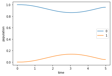
The result is the same as in the original example.

Optimize

First, we define the update shape and step width as before:

def S(t):
    """Shape function for the field update"""
    return krotov.shapes.flattop(
        t, t_start=0, t_stop=5, t_rise=0.3, t_fall=0.3, func='sinsq'
    )

pulse_options = {
    H[1][1]: dict(lambda_a=5, update_shape=S)
}

Now we can run the optimization with only small additional adjustments. This is because Krotov’s method internally does very little with the states and operators: nearly all of the numerical effort is in the propagator, which we have already defined above for the specific use of numpy arrays.

Beyond this, the optimization only needs to know three things: First, it must know how to calculate and apply the operator \(\partial H/\partial \epsilon\). We can easily teach it how to do this:

def mu(objectives, i_objective, pulses, pulses_mapping, i_pulse, time_index):
    def _mu(state):
        return H[1][0] @ state
    return _mu

Second, the pulse updates are calculated from an overlap of states, and we define an appropriate function for numpy arrays:

def overlap(psi1, psi2):
    return complex(psi1.conj().T @ psi2)

Third, it must know how to calculate the norm of states, for which we can use np.linalg.norm.

By passing all these routines to optimize_pulses, we get the exact same results as in the original example, except much faster:

opt_result = krotov.optimize_pulses(
    objectives,
    pulse_options=pulse_options,
    tlist=tlist,
    propagator=expm,
    chi_constructor=krotov.functionals.chis_re,
    info_hook=krotov.info_hooks.print_table(J_T=krotov.functionals.J_T_re),
    check_convergence=krotov.convergence.check_monotonic_error,
    iter_stop=10,
    norm=np.linalg.norm,
    mu=mu,
    overlap=overlap,
)

iter.      J_T    ∫gₐ(t)dt          J       ΔJ_T         ΔJ  secs
0     1.00e+00    0.00e+00   1.00e+00        n/a        n/a     0
1     7.65e-01    2.33e-02   7.88e-01  -2.35e-01  -2.12e-01     0
2     5.56e-01    2.07e-02   5.77e-01  -2.09e-01  -1.88e-01     0
3     3.89e-01    1.66e-02   4.05e-01  -1.67e-01  -1.51e-01     0
4     2.65e-01    1.23e-02   2.77e-01  -1.24e-01  -1.12e-01     0
5     1.78e-01    8.63e-03   1.87e-01  -8.68e-02  -7.82e-02     0
6     1.19e-01    5.86e-03   1.25e-01  -5.89e-02  -5.30e-02     0
7     8.01e-02    3.91e-03   8.40e-02  -3.92e-02  -3.53e-02     0
8     5.42e-02    2.58e-03   5.68e-02  -2.59e-02  -2.33e-02     0
9     3.71e-02    1.70e-03   3.88e-02  -1.71e-02  -1.54e-02     0
10    2.58e-02    1.13e-03   2.70e-02  -1.13e-02  -1.02e-02     0

opt_result

Krotov Optimization Result
--------------------------
- Started at 2019-12-15 22:48:47
- Number of objectives: 1
- Number of iterations: 10
- Reason for termination: Reached 10 iterations
- Ended at 2019-12-15 22:48:51 (0:00:04)